$\newcommand{\dede}[2]{\frac{\partial #1}{\partial #2} }
\newcommand{\dd}[2]{\frac{d #1}{d #2}}
\newcommand{\divby}[1]{\frac{1}{#1} }
\newcommand{\typing}[3][\Gamma]{#1 \vdash #2 : #3}
\newcommand{\xyz}[0]{(x,y,z)}
\newcommand{\xyzt}[0]{(x,y,z,t)}
\newcommand{\hams}[0]{-\frac{\hbar^2}{2m}(\dede{^2}{x^2} + \dede{^2}{y^2} + \dede{^2}{z^2}) + V\xyz}
\newcommand{\hamt}[0]{-\frac{\hbar^2}{2m}(\dede{^2}{x^2} + \dede{^2}{y^2} + \dede{^2}{z^2}) + V\xyzt}
\newcommand{\ham}[0]{-\frac{\hbar^2}{2m}(\dede{^2}{x^2}) + V(x)}
\newcommand{\konko}[2]{^{#1}\space_{#2}}
\newcommand{\kokon}[2]{_{#1}\space^{#2}} $
# Content
$\newcommand{\L}{\mathcal L}$
$\newcommand{\lrangle}[1]{\langle #1 \rangle}$
## Greens functions sidenotes
### Operator inverses
Last week I introduced greens functions as the reaction to a delta, this is technically not exactly a greens function, but rather a fundamental solution.
An other way to motivate the greens function is the other way around. Instead of claiming I want to find the response to a $\delta$. I can ask:
When is $LG = id$
Or more intuitively: $L(G(\rho)) = \rho$
So what do I need to do to my charge distribution, such that after applying the equation I get the same distribution back.
This might sound more complicated, but from a linalg perspective (note that L is gonna be a linear opearator) this is a very common problem.
What we are doing here is we are finding the inverse of $L$.
$L(L^{-1}(\rho)) = id(\rho) = \rho$
The reason why the delta approach works is because $\delta_{x,x'}$ forms a complete basis of $x$-space. We could just as well have chosen a different basis, and could have gotten a similarly useful result (keep that in mind)
### Boundary conditions
Remember last week we characterized greens functions by saying that they:
- Solve the operator for a $\delta$ inside the region
- Satisfy the boundary conditions
This was slightly simplified, because technically I only showed you how to solve for the case where the boundary condition was 0.
#### The particular solution
The reason why we cared about this special case was because now it's fairly easy to actually solve the full problem:
Let's say we have the problem:
$$L \phi = \rho$$
(That could for example be the poisson equation)
$$\Delta \phi = -\frac{\rho}{\varepsilon}$$
Now often we actually also have boundary conditions which are non-zero.
Let's say we want to solve the above problem with the additional condition that $\forall x\in \mathcal B: \phi(x) = g(x)$
Building our $\phi$ using the standard greens function approach:
$\phi = \int G(x,s) \rho(s) ds$
will however (by construction) give us $\phi(\mathcal B) = 0$ (in case we incorporated the zero boundary condition already)
##### Sidenote integration
Let's say you want to find the solution to the following problem:
$\dd{f}{x} = x^{2}$ (note that this has the exact same form as above)
We know that we can solve this problem by integrating:
$\int \dd{f}{x} - x^{2} dx= 0$
$f - \frac{1}{3}x^{3}= 0$
$f = \frac{1}{3}x^{3}$
Now imagine I wanted to also satisfy the boundary condition that $f(3) = 5$
How would I go about this?
In essence what I want is:
$\left(\dd{f}{x} - x^{2} \right)|_{x=3} = 5$
Or even: $\forall x \in \mathcal B :Lf(x) - x^{2} = g(x) = 5$
We realize that there are solutions to the specific problem:
$\dd{f}{x} - x^{2} =5$
Note that if I add constant terms to $f$ they don't even show up in the solution.
We can thus write:
$f_{p}(x) = -4$
Note how the homogeneous problem $\dd{f}{x} = 0$ is unaffected by $f_{p}$
The full solution is thus:
$f(x) = \frac{1}{3}x^{3} -4$
Plugging it into the problem we get:
$\dd{f}{x} = x^{2}$
and
$$f(3) = \frac{1}{3}3^{3} - 4 = 5$$
This is obviously a massively over complicated way to say that $\int x^{2}= \frac{1}{3}x^{3} + C$
But it shows which roles the different parts of the problem play.
- The differential operator $L$ takes the form of "the thing we want to integrate" (or more generally we want to invert)
- The initial value problem $f(3) = 5$ corresponds to the boundary value problem
- The function we integrate $x^{2}$ takes the role of the distribution $\rho$.
Sidenote, the way we found $+C$ is general for the differential operator $L = \dd{}{x}$, this is the reason why we write $+C$ in the first place.
##### Back to Green
We thus want to find something that is like the integration constant. It thus has to solve the homogeneous problem:
$L\phi = 0$
While also fulfilling the boundary problem:
$\phi(x \in \mathcal B) = g(x)$
##### Semi example
Imagine solving the poisson problem in a plate capacitor. With a plate at $x =0$ and one at $x = d$, with $\phi(0) = 0$ and $\phi(d) = 10 V$
Solving it for the case with $\phi(0) = \phi(d) = 0$, we will get some sort of "infinite mirror tunnel" mirror charge solution.
 The bondary problem now is to find a field distribution $\phi$, which solves the poisson equation for $\rho = 0$. Luckily we can simply choose a linear gradient $\phi_{p}(x) = \frac{10V}{d}\cdot x$
Which has $\Delta \phi = 0$
And $\phi(0) = 0$ , $\phi(d) = 10V$
The full solution will thus be:
$\phi_{h}(x) + \phi_{p}$
## Quantum Scattering Theory
### Lippman Schwinger
I will approach the equation from slightly different angle than the script:
We start with the SE:
$$\left[-\frac{\hbar^{2}}{2m}\nabla^{2} + V(x)\right]\psi = E\psi$$
We first want to understand what is given, and what we are looking for:
- We will be scattering waves off of a particle distribution. The distribution will be given by $V$, thus this will be the same as $\rho$ in the poisson equation
- The waves will have varying energies and come from infinity. This will give us some sort of boundary conditions.
We rearrange the equation to get the more familiar $L\phi = \rho$ form:
$$\left(\frac{\hbar^{2}}{2m}\nabla^{2}+E\right)\psi = V\psi$$
We note some slight differences between this and the poisson equation:
1) We find $\psi$ on both sides
2) We have this $-E$ term, which is thus far unspecified.
We'll realize that having $\psi$ on the RHS is not such a big deal.
##### Inhomogeneous
We want to show that a greens function will be good enough to solve the problem even with the $\psi$ on both sides
$$\left(\frac{\hbar^{2}}{2m}\nabla^{2} + E\right)G(\vec x,\vec s) =^{!} \delta(\vec x, \vec s)$$
We can reconstruct the RHS using this approach:
$$ \int \left(\frac{\hbar^{2}}{2m}\nabla^{2} + E\right)G(x,s) f(s) ds = f(x)$$
$$ \int \left(\frac{\hbar^{2}}{2m}\nabla_{x}^{2} + E\right)G(x,s) V(s)\psi(s) ds = V(x)\psi(x)$$
Using the linearity of the integral we can take out the operator $L$.
$$\left(\frac{\hbar^{2}}{2m}\nabla_{x}^{2} + E\right) \underbrace{\int G(x,s) V(s)\psi(s) ds}_{\psi} = V(x)\psi(x)$$
We recognize the form of the original equation.
We can thus say:
$$\int G(x,s) V(s)\psi(s) ds = \psi(x)$$
This solves the problem for the scattering object, but it doesn't solve the boundary conditions (we want the possiblility to add waves to the problem)
##### Homogeneous
We thus solve the homogeneous problem with boundary conditions:
$$\left(\frac{\hbar^{2}}{2m}\nabla^{2}+E\right)\psi = 0$$
This should be fairly familiar to you from electrodynamics. this is a wave equation:
$\psi = e^{i\vec k \vec x}$
With $E_{k}= \frac{\hbar^{2}k^{2}}{2m}$
What this means is that we can find the "Energy initial value problem" (or the initial wave problem) in the case where we don't have anything to scatter of off
##### Full solution
The full solution is the so-called lippman schwinger equation:
$$\psi_{k}(x) = \int G_{k}(x-s)V(s)\psi_{k}(s) ds + e^{ikx}$$
Now the thing is that this is not really better than what we started with...
Arguably it's even worse! We have an integral now and also this unknown greens function.
##### Solving for G
We can use a well known trick for solving PDE's now: Fourier transform:
$$G_{k}(x) = \frac{1}{(2\pi)^{3}}\int G_{k}(q)e^{iqx} d^{3}q$$
Plugging this into the defining function for $G$ and applying the $\nabla$ to $G$ we get:
$$\frac{1}{{(2\pi)^{3}}} \int \left(-\frac{\hbar^{2}}{2m}q^{2} + E_{k}\right) G_{k}(q)e^{iqx} d^{3}q = \delta(x)$$
Which of course still need to satisfy the delta condition.
Writing both sides in the fourier domain we get
$$\frac{1}{{(2\pi)^{3}}} \int \left(-\frac{\hbar^{2}}{2m}q^{2} + E_{k}\right) G_{k}(q)e^{iqx} d^{3}q = \frac{1}{(2\pi)^{3}}\int e^{iqx} d^{3}q$$
Comparing coefficients we find:
$G_{k}(q) = \frac{1}{E_{k}- \frac{\hbar^{2}q^{2}}{2m}}$
Or simply
$G_{k}(q) = \frac{2m}{\hbar^{2}} \frac{1}{k^{2}-q^{2}}$
Fourier transforming back is not entirely trivial, because we have a pole for $k=q$ and one for $k = -q$
Doing some complex analysis we end up with:
$G_{k}(x) = - \frac{m}{2\pi \hbar^{2}} \frac{e^{ikr}}{r}$
This is actually not entirely surprising when considering how close it is to the poisson equation. The only real difference between the poisson equation and this is the energy term, which manifests as a shift by $\sim k$ in the fourier domain. Shifting in the fourier domain corresponds to a phase factor. The kernel is thus the well known $\frac{1}{r}$ solution for the poisson equation, with a corresponding $e^{ikr}$ phase factor.
Plugging this back in we get:
The bondary problem now is to find a field distribution $\phi$, which solves the poisson equation for $\rho = 0$. Luckily we can simply choose a linear gradient $\phi_{p}(x) = \frac{10V}{d}\cdot x$
Which has $\Delta \phi = 0$
And $\phi(0) = 0$ , $\phi(d) = 10V$
The full solution will thus be:
$\phi_{h}(x) + \phi_{p}$
## Quantum Scattering Theory
### Lippman Schwinger
I will approach the equation from slightly different angle than the script:
We start with the SE:
$$\left[-\frac{\hbar^{2}}{2m}\nabla^{2} + V(x)\right]\psi = E\psi$$
We first want to understand what is given, and what we are looking for:
- We will be scattering waves off of a particle distribution. The distribution will be given by $V$, thus this will be the same as $\rho$ in the poisson equation
- The waves will have varying energies and come from infinity. This will give us some sort of boundary conditions.
We rearrange the equation to get the more familiar $L\phi = \rho$ form:
$$\left(\frac{\hbar^{2}}{2m}\nabla^{2}+E\right)\psi = V\psi$$
We note some slight differences between this and the poisson equation:
1) We find $\psi$ on both sides
2) We have this $-E$ term, which is thus far unspecified.
We'll realize that having $\psi$ on the RHS is not such a big deal.
##### Inhomogeneous
We want to show that a greens function will be good enough to solve the problem even with the $\psi$ on both sides
$$\left(\frac{\hbar^{2}}{2m}\nabla^{2} + E\right)G(\vec x,\vec s) =^{!} \delta(\vec x, \vec s)$$
We can reconstruct the RHS using this approach:
$$ \int \left(\frac{\hbar^{2}}{2m}\nabla^{2} + E\right)G(x,s) f(s) ds = f(x)$$
$$ \int \left(\frac{\hbar^{2}}{2m}\nabla_{x}^{2} + E\right)G(x,s) V(s)\psi(s) ds = V(x)\psi(x)$$
Using the linearity of the integral we can take out the operator $L$.
$$\left(\frac{\hbar^{2}}{2m}\nabla_{x}^{2} + E\right) \underbrace{\int G(x,s) V(s)\psi(s) ds}_{\psi} = V(x)\psi(x)$$
We recognize the form of the original equation.
We can thus say:
$$\int G(x,s) V(s)\psi(s) ds = \psi(x)$$
This solves the problem for the scattering object, but it doesn't solve the boundary conditions (we want the possiblility to add waves to the problem)
##### Homogeneous
We thus solve the homogeneous problem with boundary conditions:
$$\left(\frac{\hbar^{2}}{2m}\nabla^{2}+E\right)\psi = 0$$
This should be fairly familiar to you from electrodynamics. this is a wave equation:
$\psi = e^{i\vec k \vec x}$
With $E_{k}= \frac{\hbar^{2}k^{2}}{2m}$
What this means is that we can find the "Energy initial value problem" (or the initial wave problem) in the case where we don't have anything to scatter of off
##### Full solution
The full solution is the so-called lippman schwinger equation:
$$\psi_{k}(x) = \int G_{k}(x-s)V(s)\psi_{k}(s) ds + e^{ikx}$$
Now the thing is that this is not really better than what we started with...
Arguably it's even worse! We have an integral now and also this unknown greens function.
##### Solving for G
We can use a well known trick for solving PDE's now: Fourier transform:
$$G_{k}(x) = \frac{1}{(2\pi)^{3}}\int G_{k}(q)e^{iqx} d^{3}q$$
Plugging this into the defining function for $G$ and applying the $\nabla$ to $G$ we get:
$$\frac{1}{{(2\pi)^{3}}} \int \left(-\frac{\hbar^{2}}{2m}q^{2} + E_{k}\right) G_{k}(q)e^{iqx} d^{3}q = \delta(x)$$
Which of course still need to satisfy the delta condition.
Writing both sides in the fourier domain we get
$$\frac{1}{{(2\pi)^{3}}} \int \left(-\frac{\hbar^{2}}{2m}q^{2} + E_{k}\right) G_{k}(q)e^{iqx} d^{3}q = \frac{1}{(2\pi)^{3}}\int e^{iqx} d^{3}q$$
Comparing coefficients we find:
$G_{k}(q) = \frac{1}{E_{k}- \frac{\hbar^{2}q^{2}}{2m}}$
Or simply
$G_{k}(q) = \frac{2m}{\hbar^{2}} \frac{1}{k^{2}-q^{2}}$
Fourier transforming back is not entirely trivial, because we have a pole for $k=q$ and one for $k = -q$
Doing some complex analysis we end up with:
$G_{k}(x) = - \frac{m}{2\pi \hbar^{2}} \frac{e^{ikr}}{r}$
This is actually not entirely surprising when considering how close it is to the poisson equation. The only real difference between the poisson equation and this is the energy term, which manifests as a shift by $\sim k$ in the fourier domain. Shifting in the fourier domain corresponds to a phase factor. The kernel is thus the well known $\frac{1}{r}$ solution for the poisson equation, with a corresponding $e^{ikr}$ phase factor.
Plugging this back in we get:
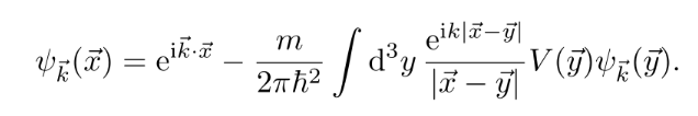 We now assume that $V$ is short ranged, that means that we can approximate the integral to have finite support.
The impact of the Green's function when we use it only on finite support decays as $\frac{1}{r}$. The distance from the particle to the detector $x$ and the distance between particle and potential $y$ thus have: $y\ll x$
$|x-y| = \sqrt{(x-y)^{2}} = \sqrt{x^{2} + y^{2} - 2xy} = r \sqrt{1 + \frac{y^{2}}{r^{2}}- \frac{2xy}{r^{2}}}$
$$|x-y| \approx r - \frac{x\cdot y}{r}$$
We now do a slightly strange move. We use this approximation for the exponent, but not for the fraction.
For the fraction we will actually use the even simpler $|x-y| \approx r$
Physically we can think of this as follows:
- For the phase (interference and such) the relevant order of accuracy is $k$, since $\frac{1}{k}$ (the wavelength) will very probably be close to $y$ we need to be quite accurate,
- For the decay we don't really care about the $y$, since the relevant comparison here is to $x$.
Thus we get:
$\psi_{k}(x) = e^{ikx} + \frac{e^{ikx}}{r} f(k,k')$
With
$$f(k,k') = - \frac{m}{2\pi\hbar^{2}}\int e^{-ik's}V(s)\psi_{k}(s) d^{3}s$$
With $k' = \frac{kx}{r}$
$f$ is called the scattering amplitude.
We now try to understand the equation:
We now assume that $V$ is short ranged, that means that we can approximate the integral to have finite support.
The impact of the Green's function when we use it only on finite support decays as $\frac{1}{r}$. The distance from the particle to the detector $x$ and the distance between particle and potential $y$ thus have: $y\ll x$
$|x-y| = \sqrt{(x-y)^{2}} = \sqrt{x^{2} + y^{2} - 2xy} = r \sqrt{1 + \frac{y^{2}}{r^{2}}- \frac{2xy}{r^{2}}}$
$$|x-y| \approx r - \frac{x\cdot y}{r}$$
We now do a slightly strange move. We use this approximation for the exponent, but not for the fraction.
For the fraction we will actually use the even simpler $|x-y| \approx r$
Physically we can think of this as follows:
- For the phase (interference and such) the relevant order of accuracy is $k$, since $\frac{1}{k}$ (the wavelength) will very probably be close to $y$ we need to be quite accurate,
- For the decay we don't really care about the $y$, since the relevant comparison here is to $x$.
Thus we get:
$\psi_{k}(x) = e^{ikx} + \frac{e^{ikx}}{r} f(k,k')$
With
$$f(k,k') = - \frac{m}{2\pi\hbar^{2}}\int e^{-ik's}V(s)\psi_{k}(s) d^{3}s$$
With $k' = \frac{kx}{r}$
$f$ is called the scattering amplitude.
We now try to understand the equation:
 We can now think about how much of the wave interacted with our scatterer (the differential cross-section).
We notice that in spherical coordinates the incoming wave is just one point, everywhere else we only see the outgoing circular wave. (Note that the $\frac{1}{r}$ factor canceles the $r$ from the spherical coordinates)
Thus the spherical wave part (or more accurately $f$) will be the "magnitude" of the scattered wave. Because we need a real probabiliyt and $f$ works on wavefunctions, we need $|f|^{2}$
Thus we get:
$$\dd{\sigma}{\Omega}(k,k') = |f(k,k')|^{2}$$
This is true except for $k = k'$, where we also need to consider the original beam.
### Born approximation
Note how the LS equation still gives no concrete way how to solve for $\psi$ (which occurs both as the solution, as well as in the input to $f$)
We realize however, that we could solve $\psi$ recursively, by plugging the LS equation into itself repeatedly.
We define the LS-operator:
$K\psi = \int G_{k}(x-s) V(s) \psi(s)d^{3}s$
The LS equation is thus:
$$\psi = \underbrace{e^{ikx}}_{\phi} + K\psi$$
$$\psi_{k}= (1+K + \ldots + K^{n}) \phi + K^{n+1}\psi$$
Where $K$ introduces values of the order of $V$. (we kind of multiply by the potential).
If the potential is small, each application will be less and less important, as it picks up the $V$ factor.
Capping the equation at the first term we get the Born approximation:
$\psi = (1+ K)\phi$
Physically this means, that the wave only interacts once, and then escapes. There are no such things as a double scattering. This is why we can just input the plane wave $\phi$
In this approximation $f$ is actually solvable:
We can now think about how much of the wave interacted with our scatterer (the differential cross-section).
We notice that in spherical coordinates the incoming wave is just one point, everywhere else we only see the outgoing circular wave. (Note that the $\frac{1}{r}$ factor canceles the $r$ from the spherical coordinates)
Thus the spherical wave part (or more accurately $f$) will be the "magnitude" of the scattered wave. Because we need a real probabiliyt and $f$ works on wavefunctions, we need $|f|^{2}$
Thus we get:
$$\dd{\sigma}{\Omega}(k,k') = |f(k,k')|^{2}$$
This is true except for $k = k'$, where we also need to consider the original beam.
### Born approximation
Note how the LS equation still gives no concrete way how to solve for $\psi$ (which occurs both as the solution, as well as in the input to $f$)
We realize however, that we could solve $\psi$ recursively, by plugging the LS equation into itself repeatedly.
We define the LS-operator:
$K\psi = \int G_{k}(x-s) V(s) \psi(s)d^{3}s$
The LS equation is thus:
$$\psi = \underbrace{e^{ikx}}_{\phi} + K\psi$$
$$\psi_{k}= (1+K + \ldots + K^{n}) \phi + K^{n+1}\psi$$
Where $K$ introduces values of the order of $V$. (we kind of multiply by the potential).
If the potential is small, each application will be less and less important, as it picks up the $V$ factor.
Capping the equation at the first term we get the Born approximation:
$\psi = (1+ K)\phi$
Physically this means, that the wave only interacts once, and then escapes. There are no such things as a double scattering. This is why we can just input the plane wave $\phi$
In this approximation $f$ is actually solvable:
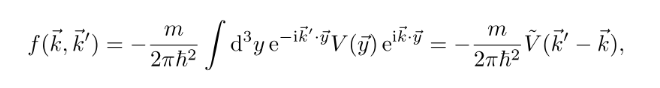 And corresponds to the fourier transform of our potential. (this is basically fully analogous to the hygens principle)
## Recap continuation
Last week in the recap we found the path integral:
And corresponds to the fourier transform of our potential. (this is basically fully analogous to the hygens principle)
## Recap continuation
Last week in the recap we found the path integral:
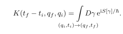 Which we found then by solving explicitly for the short time propagator kernel (greens function) and concatenating the solutions via the path integral.
In the lecture we then looked at how we can understand this path integral
### Understanding the path integral
We saw that we can now map solutions of classical problems to those of quantum problems by including the classical action along a path as the phase of the path.
We saw that for paths with similar actions (on the order of $\hbar$) we got constructive interference.
### The classical limit
We wanted to narrow that intuition and considered a path that is close to the classical path.
In the exercises you saw that for this case we got that the action along this perturbed path is very close to the classical path.
This was a consequence from the extremalisation principle of the classical path:
Remember: When finding the classical path we do this by saying that $S[\gamma + h]$ should be independent of $h$.
But our quantum perturbation is exactly such an $h$.
Thus the paths that are close to the classical path are exactly the paths that will constructively interfer.
#### Euclidean path integral
We now get a new perspective on this statement. When we replace the $e^{\frac{iS[\gamma]}{\hbar}}$ with $e^{\frac{-S_{E}[\gamma]}{\hbar}}$
We see that the paths that exremalize the action (minimize) will be the strongest contributions! You'll see this in statistical physics under the name of saddle point integration.
#### Classical limit
In the classical limit the oscillations get smaller and smaller, thus the "radius of interference" also gets smaller and smaller. We get less tollerance for "almost optimal " paths.
In the limit we obtain exactly the classical paths
### Commutation & Time ordering
We then wanted to find whether this new quantum formalism was compatible with the old formalism of canonical quantisation:
For this we wanted to explicitly compute the commutator.
We found a small problem when doing this, which was that we had "non-causal" or time reversed measurements.
We thus needed to find how to "time order" our operators.
After doing some BCH reformulations we found that our formalism was indeed compatible with canonical quantisation
Which we found then by solving explicitly for the short time propagator kernel (greens function) and concatenating the solutions via the path integral.
In the lecture we then looked at how we can understand this path integral
### Understanding the path integral
We saw that we can now map solutions of classical problems to those of quantum problems by including the classical action along a path as the phase of the path.
We saw that for paths with similar actions (on the order of $\hbar$) we got constructive interference.
### The classical limit
We wanted to narrow that intuition and considered a path that is close to the classical path.
In the exercises you saw that for this case we got that the action along this perturbed path is very close to the classical path.
This was a consequence from the extremalisation principle of the classical path:
Remember: When finding the classical path we do this by saying that $S[\gamma + h]$ should be independent of $h$.
But our quantum perturbation is exactly such an $h$.
Thus the paths that are close to the classical path are exactly the paths that will constructively interfer.
#### Euclidean path integral
We now get a new perspective on this statement. When we replace the $e^{\frac{iS[\gamma]}{\hbar}}$ with $e^{\frac{-S_{E}[\gamma]}{\hbar}}$
We see that the paths that exremalize the action (minimize) will be the strongest contributions! You'll see this in statistical physics under the name of saddle point integration.
#### Classical limit
In the classical limit the oscillations get smaller and smaller, thus the "radius of interference" also gets smaller and smaller. We get less tollerance for "almost optimal " paths.
In the limit we obtain exactly the classical paths
### Commutation & Time ordering
We then wanted to find whether this new quantum formalism was compatible with the old formalism of canonical quantisation:
For this we wanted to explicitly compute the commutator.
We found a small problem when doing this, which was that we had "non-causal" or time reversed measurements.
We thus needed to find how to "time order" our operators.
After doing some BCH reformulations we found that our formalism was indeed compatible with canonical quantisation