$\newcommand{\dede}[2]{\frac{\partial #1}{\partial #2} }
\newcommand{\dd}[2]{\frac{d #1}{d #2}}
\newcommand{\divby}[1]{\frac{1}{#1} }
\newcommand{\typing}[3][\Gamma]{#1 \vdash #2 : #3}
\newcommand{\xyz}[0]{(x,y,z)}
\newcommand{\xyzt}[0]{(x,y,z,t)}
\newcommand{\hams}[0]{-\frac{\hbar^2}{2m}(\dede{^2}{x^2} + \dede{^2}{y^2} + \dede{^2}{z^2}) + V\xyz}
\newcommand{\hamt}[0]{-\frac{\hbar^2}{2m}(\dede{^2}{x^2} + \dede{^2}{y^2} + \dede{^2}{z^2}) + V\xyzt}
\newcommand{\ham}[0]{-\frac{\hbar^2}{2m}(\dede{^2}{x^2}) + V(x)}
\newcommand{\konko}[2]{^{#1}\space_{#2}}
\newcommand{\kokon}[2]{_{#1}\space^{#2}} $
# Content
$\newcommand{\L}{\mathcal L}$
$\newcommand{\lrangle}[1]{\langle #1 \rangle}$
## Continuation euclidian path integrals
The last time we found out that we can equate thermal distributions with path integrals in complex time
$$\lrangle A_{\beta} = \frac{1}{Z}\int d_{q}\int_{\substack{i\hbar \frac{\beta}{2}\to -i\hbar \frac{\beta}{2} \\ q \to q}} D\gamma A(\gamma(0)) e^{\frac{iS[\gamma]}{\hbar}}$$
This was basically a trick to reformulate the thermal integral of type $e^{-\beta H}$ to a path integral.
We didn't end at that point however. We made an additional step to get rid of the complex time integration. We introduced the euclidean time.
$\tau = it$
We found:
$$\lrangle A = \frac{1}{Z} \int_{\text{cyclic length }\beta\hbar} D\gamma A(\gamma_{E}(0))e^{\frac{-S_{E}[\gamma_{E}]}{\hbar}}$$
Mathematically we can also see this as a rotation of our entire problem:
 ## Primer scattering theory
When investigating smaller and smaller objects direct observation quickly becomes impossible. This phenomenon is already evident at intermediary scales.
One example which is "almost not even quantum" is the electron microscope.
To picture structures which are smaller than wavelengths of visible light we need something that has even shorter wavelengths. One way to acheive thist this is to use higher energy light, such as X-rays. However X-rays are often very destructive to structures we want to observe.
The alternative path is by using the wave particle duality, and using massive particles.
The advantage is, as you saw in the classical limit of the path integral, that the mass of an object gives you "free fast oscillations". That means that even much slower electrons will have much shorter wavelenghts.
The real use case for scattering theory in modern physics however is high-energy particle physics, where we can probe interactions via scattering.
### Classical scattering theory:
## Primer scattering theory
When investigating smaller and smaller objects direct observation quickly becomes impossible. This phenomenon is already evident at intermediary scales.
One example which is "almost not even quantum" is the electron microscope.
To picture structures which are smaller than wavelengths of visible light we need something that has even shorter wavelengths. One way to acheive thist this is to use higher energy light, such as X-rays. However X-rays are often very destructive to structures we want to observe.
The alternative path is by using the wave particle duality, and using massive particles.
The advantage is, as you saw in the classical limit of the path integral, that the mass of an object gives you "free fast oscillations". That means that even much slower electrons will have much shorter wavelenghts.
The real use case for scattering theory in modern physics however is high-energy particle physics, where we can probe interactions via scattering.
### Classical scattering theory:

 The main idea behind scattering theory is mapping the geometry of an input scatterer to the geometry of the output.
For this we first consider a ray of particles hitting a fixed object.
- What are the correct symmetries to describe the situation above?
We see that we have essentially two parts of the problem, each with their individual symmetry:
- Ray: Cylindrical symmetry
- Particle: Spherical symmetry
Now even if the particle is not round, it makes sense to start from a round particle and then start perturbing it. If you remember MMP I you might remember the spherical harmonics. You can always expand your object in these, which will turn out to be useful. We'll talk later about this in the course.
#### Differential cross section
As we saw in the above picture if we want to describe scattering we need to have some object that translates things (we will mostly consider particle or energy fluxes) from the "ray frame" to the "sphere frame"
The object we are looking for is the differential cross section:
$$\dd{\sigma}{\Omega}$$
It specifies the input area needed to span a certain output solid angle. Note that the units are different. We have an area divided by a solid angle.
Also note that this value can be computed at any point of the output sphere. We can imagine it as follows:
Put a detector covering some solid angle on the output sphere. The differential cross section tells me what fraction of the total beam power ends up being scattered into that detector. It thus has to be a function of the output coordinates $\theta$ and $\phi$
If I integrate over the full sphere I should also get the full input beam power back.
#### Why differential cross section
The differential cross section contains a lot of information about the "shape" of the object.
Imagine you find that your beam is deflected only onto a narrow ring. Which of the two shapes would you expect to be responsible for this?
The main idea behind scattering theory is mapping the geometry of an input scatterer to the geometry of the output.
For this we first consider a ray of particles hitting a fixed object.
- What are the correct symmetries to describe the situation above?
We see that we have essentially two parts of the problem, each with their individual symmetry:
- Ray: Cylindrical symmetry
- Particle: Spherical symmetry
Now even if the particle is not round, it makes sense to start from a round particle and then start perturbing it. If you remember MMP I you might remember the spherical harmonics. You can always expand your object in these, which will turn out to be useful. We'll talk later about this in the course.
#### Differential cross section
As we saw in the above picture if we want to describe scattering we need to have some object that translates things (we will mostly consider particle or energy fluxes) from the "ray frame" to the "sphere frame"
The object we are looking for is the differential cross section:
$$\dd{\sigma}{\Omega}$$
It specifies the input area needed to span a certain output solid angle. Note that the units are different. We have an area divided by a solid angle.
Also note that this value can be computed at any point of the output sphere. We can imagine it as follows:
Put a detector covering some solid angle on the output sphere. The differential cross section tells me what fraction of the total beam power ends up being scattered into that detector. It thus has to be a function of the output coordinates $\theta$ and $\phi$
If I integrate over the full sphere I should also get the full input beam power back.
#### Why differential cross section
The differential cross section contains a lot of information about the "shape" of the object.
Imagine you find that your beam is deflected only onto a narrow ring. Which of the two shapes would you expect to be responsible for this?
 We see that for solid objects the curvature is the relevant factor to determine the differential cross section.
The differential cross section also contains information about the size of the object.
This connection is a bit more subtle, but essentially we have thus far assumed that the ray covers the full scatterer uniformly. But we can actually also formulate our cross section with input and output variables. This then allows us to find cutoffs for when a ray getting larger will no longer give significant contributions to the cross section. At this point the ray size has exceeded the sphere of influence of the scatterer.
### Quantum
In the quantum case we can no longer do the 1:1 matching of input to output. However we can still talk about the probability to find a particle in one output given it was a certain input.
The fundamental thing we want to map is thus the probability flux.
#### Repetition probability flux/ current
We remember from Physics III that $\rho(x) = |\Psi|^{2}$ for a single particle, without loss of generality this is the situation we will consider today.
Now we want to figure out the change in particle number over time:
$\partial_{t} \rho = \partial_{t}\Psi \Psi^{\star} = \Psi \Psi^{\star\prime} + \Psi^{\prime} \Psi^{\star}$
We remember the schrödinger equation equation:
$i\hbar \partial_{t} \Psi = H \Psi$
For a free particle we thus get:
$i\hbar \partial_{t} \Psi = -\frac{\hbar^{2}}{2m} \Psi$
$\partial_{t} \Psi = -\frac{\hbar}{2im} \nabla\Psi$
Thus plugging in we get:
$\partial_{t} \rho = \partial_{t}(\Psi \Psi^{\star}) = \Psi (\frac{\hbar}{2im}\nabla\Psi^{\star}) - \frac{\hbar}{2im}\nabla\Psi \Psi^{\star}$
$$\partial_{t} \rho = \partial_{t}(\Psi \Psi^{\star}) = -\frac{i\hbar}{2m}(\Psi\nabla\Psi^{\star} - \Psi^{\star}\nabla\Psi)$$
Which "coincidentally" is the probability current
$\partial_{t}\rho = -\nabla j$
This is the continuity equation. (We can even say the continuity equation defines our shape of the probability current)
> Side note about the name: If we imagine the particles to be charged, we can immediately see that this definition (simply by multiplying by the charge) also gives us the electrodynamics current continuity equation. $j$ is thus actually a current, which is simply lacking a charge.
## Greens functions repetition
For those who have taken electrodynamics or MMP I, you might remember the concept of Greens functions.
We want to solve a problem (i.e. a differential equation) on some distribution of objects (most often a density of stuff), while satisfying the boundary values of the problem.
The greens function is a useful concept to solve those types of problems, it works as follows:
- Solve the problem for a single delta-point (often without boundary)
- Fix the values on the boundary by introducing "mirror charges"
- This is the greens function
To now solve a general problem we can note that any density distribution $\rho$ can be written as: $\rho(x) = \int \delta_{x,x'} \rho(x') dx'$
For linear problems this essentially solves our full problem, because now we can simply construct our solution for $\rho$ from the small delta peaks, for which we know the solution via the greens function.
### Greens functions in action
The classical example for greens functions in action is the potential of a charge distribution $\rho$ close to a conducting plate.
We see that for solid objects the curvature is the relevant factor to determine the differential cross section.
The differential cross section also contains information about the size of the object.
This connection is a bit more subtle, but essentially we have thus far assumed that the ray covers the full scatterer uniformly. But we can actually also formulate our cross section with input and output variables. This then allows us to find cutoffs for when a ray getting larger will no longer give significant contributions to the cross section. At this point the ray size has exceeded the sphere of influence of the scatterer.
### Quantum
In the quantum case we can no longer do the 1:1 matching of input to output. However we can still talk about the probability to find a particle in one output given it was a certain input.
The fundamental thing we want to map is thus the probability flux.
#### Repetition probability flux/ current
We remember from Physics III that $\rho(x) = |\Psi|^{2}$ for a single particle, without loss of generality this is the situation we will consider today.
Now we want to figure out the change in particle number over time:
$\partial_{t} \rho = \partial_{t}\Psi \Psi^{\star} = \Psi \Psi^{\star\prime} + \Psi^{\prime} \Psi^{\star}$
We remember the schrödinger equation equation:
$i\hbar \partial_{t} \Psi = H \Psi$
For a free particle we thus get:
$i\hbar \partial_{t} \Psi = -\frac{\hbar^{2}}{2m} \Psi$
$\partial_{t} \Psi = -\frac{\hbar}{2im} \nabla\Psi$
Thus plugging in we get:
$\partial_{t} \rho = \partial_{t}(\Psi \Psi^{\star}) = \Psi (\frac{\hbar}{2im}\nabla\Psi^{\star}) - \frac{\hbar}{2im}\nabla\Psi \Psi^{\star}$
$$\partial_{t} \rho = \partial_{t}(\Psi \Psi^{\star}) = -\frac{i\hbar}{2m}(\Psi\nabla\Psi^{\star} - \Psi^{\star}\nabla\Psi)$$
Which "coincidentally" is the probability current
$\partial_{t}\rho = -\nabla j$
This is the continuity equation. (We can even say the continuity equation defines our shape of the probability current)
> Side note about the name: If we imagine the particles to be charged, we can immediately see that this definition (simply by multiplying by the charge) also gives us the electrodynamics current continuity equation. $j$ is thus actually a current, which is simply lacking a charge.
## Greens functions repetition
For those who have taken electrodynamics or MMP I, you might remember the concept of Greens functions.
We want to solve a problem (i.e. a differential equation) on some distribution of objects (most often a density of stuff), while satisfying the boundary values of the problem.
The greens function is a useful concept to solve those types of problems, it works as follows:
- Solve the problem for a single delta-point (often without boundary)
- Fix the values on the boundary by introducing "mirror charges"
- This is the greens function
To now solve a general problem we can note that any density distribution $\rho$ can be written as: $\rho(x) = \int \delta_{x,x'} \rho(x') dx'$
For linear problems this essentially solves our full problem, because now we can simply construct our solution for $\rho$ from the small delta peaks, for which we know the solution via the greens function.
### Greens functions in action
The classical example for greens functions in action is the potential of a charge distribution $\rho$ close to a conducting plate.
 We know from electrodynamics that:
$\nabla \cdot E = \frac{\rho}{\varepsilon}$
$-\nabla \phi = E$
Thus we get the poisson equation:
$$\Delta \phi = -\frac{\rho}{\varepsilon}$$
If we can solve this equation for $\rho(r) = \delta(r-r_{0})$ we could reconstruct the full solution from there.
#### Full solution:
We Fourier transform the problem:
$-k^{2}\phi = e^{-2\pi i r_{0}k}\frac{1}{\varepsilon}$
$\phi = -\frac{1}{k^{2}\varepsilon} e^{-2\pi i r_{0}k}$
Fourier transforming back we obtain:
$\phi(r) = \frac{1}{4\pi\varepsilon|r-r_{0}|}$
We now say this potential is the Greens function:
$$G(r,r_{0}) = \frac{1}{4\pi\varepsilon|r-r_{0}|}$$
##### But wait!
We have not yet solved the boundary conditions, which state that at $r=0$ the potential should be zero.
We now invent a mirror charge at $-r_{0}$ with opposite charge. This will cancle the potential on the surface.
We know from electrodynamics that:
$\nabla \cdot E = \frac{\rho}{\varepsilon}$
$-\nabla \phi = E$
Thus we get the poisson equation:
$$\Delta \phi = -\frac{\rho}{\varepsilon}$$
If we can solve this equation for $\rho(r) = \delta(r-r_{0})$ we could reconstruct the full solution from there.
#### Full solution:
We Fourier transform the problem:
$-k^{2}\phi = e^{-2\pi i r_{0}k}\frac{1}{\varepsilon}$
$\phi = -\frac{1}{k^{2}\varepsilon} e^{-2\pi i r_{0}k}$
Fourier transforming back we obtain:
$\phi(r) = \frac{1}{4\pi\varepsilon|r-r_{0}|}$
We now say this potential is the Greens function:
$$G(r,r_{0}) = \frac{1}{4\pi\varepsilon|r-r_{0}|}$$
##### But wait!
We have not yet solved the boundary conditions, which state that at $r=0$ the potential should be zero.
We now invent a mirror charge at $-r_{0}$ with opposite charge. This will cancle the potential on the surface.
 The full Greens function is thus:
$$G(r,r_{0}) = \frac{1}{4\pi\varepsilon|r-r_{0}|} -\frac{1}{4\pi\varepsilon|r-(-r_{0}^{x}, r_{0}^{y}, r_{0}^{z})|} $$
This potential looks as follows:
The full Greens function is thus:
$$G(r,r_{0}) = \frac{1}{4\pi\varepsilon|r-r_{0}|} -\frac{1}{4\pi\varepsilon|r-(-r_{0}^{x}, r_{0}^{y}, r_{0}^{z})|} $$
This potential looks as follows:
 We can now find the full solution by convolving our Greens function with our charge distribution:
$$\phi(r) = \int \rho(r')G(r,r') dr'$$
We can think about this like a brush in a digital art program. $G$ is the shape of the brush and $\rho$ is the lines I draw.
### Greens function in scattering
We will need greens functions for scattering because:
- QM is linear
- Objects might be more and more complicated
- Scattering of a delta peak is easy
### Greens function in path integral formalism
Do you remember any other objects with the property that they solved some differential equation for point particles, and then extended it to densities of said delta points?
...
Exactly when we solved the path integral formalism this is exactly what we did with the propagator kernel:
- We had a differential equation (the schrödinger equation)
- That we wanted to solve on a domain (either free propagation or propagation through a slit)
- And where we could reconstruct the solution for densities by convolving a greens function with the density.
Note:
$$\phi(r) = \int G(r,r') \rho(r') dr'$$
and
$$\psi(\tilde r , \tilde t) = \int K(r,\tilde r, t, \tilde t) \psi(r,t) dr dt$$
## Recap continuation
Last week in the recap we found the path integral:
We can now find the full solution by convolving our Greens function with our charge distribution:
$$\phi(r) = \int \rho(r')G(r,r') dr'$$
We can think about this like a brush in a digital art program. $G$ is the shape of the brush and $\rho$ is the lines I draw.
### Greens function in scattering
We will need greens functions for scattering because:
- QM is linear
- Objects might be more and more complicated
- Scattering of a delta peak is easy
### Greens function in path integral formalism
Do you remember any other objects with the property that they solved some differential equation for point particles, and then extended it to densities of said delta points?
...
Exactly when we solved the path integral formalism this is exactly what we did with the propagator kernel:
- We had a differential equation (the schrödinger equation)
- That we wanted to solve on a domain (either free propagation or propagation through a slit)
- And where we could reconstruct the solution for densities by convolving a greens function with the density.
Note:
$$\phi(r) = \int G(r,r') \rho(r') dr'$$
and
$$\psi(\tilde r , \tilde t) = \int K(r,\tilde r, t, \tilde t) \psi(r,t) dr dt$$
## Recap continuation
Last week in the recap we found the path integral:
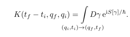 Which we found then by solving explicitly for the short time propagator kernel (greens function) and concatenating the solutions via the path integral.
In the lecture we then looked at how we can understand this path integral
### Understanding the path integral
We saw that we can now map solutions of classical problems to those of quantum problems by including the classical action along a path as the phase of the path.
We saw that for paths with similar actions (on the order of $\hbar$) we got constructive interference.
### The classical limit
We wanted to narrow that intuition and considered a path that is close to the classical path.
In the exercises you saw that for this case we got that the action along this perturbed path is very close to the classical path.
This was a consequence from the extremalisation principle of the classical path:
Remember: When finding the classical path we do this by saying that $S[\gamma + h]$ should be independent of $h$.
But our quantum perturbation is exactly such an $h$.
Thus the paths that are close to the classical path are exactly the paths that will constructively interfer.
#### Euclidean path integral
We now get a new perspective on this statement. When we replace the $e^{\frac{iS[\gamma]}{\hbar}}$ with $e^{\frac{-S_{E}[\gamma]}{\hbar}}$
We see that the paths that exremalize the action (minimize) will be the strongest contributions! You'll see this in statistical physics under the name of saddle point integration.
#### Classical limit
In the classical limit the oscillations get smaller and smaller, thus the "radius of interference" also gets smaller and smaller. We get less tollerance for "almost optimal " paths.
In the limit we obtain exactly the classical paths
### Commutation & Time ordering
We then wanted to find whether this new quantum formalism was compatible with the old formalism of canonical quantisation:
For this we wanted to explicitly compute the commutator.
We found a small problem when doing this, which was that we had "non-causal" or time reversed measurements.
We thus needed to find how to "time order" our operators.
After doing some BCH reformulations we found that our formalism was indeed compatible with canonical quantisation
Which we found then by solving explicitly for the short time propagator kernel (greens function) and concatenating the solutions via the path integral.
In the lecture we then looked at how we can understand this path integral
### Understanding the path integral
We saw that we can now map solutions of classical problems to those of quantum problems by including the classical action along a path as the phase of the path.
We saw that for paths with similar actions (on the order of $\hbar$) we got constructive interference.
### The classical limit
We wanted to narrow that intuition and considered a path that is close to the classical path.
In the exercises you saw that for this case we got that the action along this perturbed path is very close to the classical path.
This was a consequence from the extremalisation principle of the classical path:
Remember: When finding the classical path we do this by saying that $S[\gamma + h]$ should be independent of $h$.
But our quantum perturbation is exactly such an $h$.
Thus the paths that are close to the classical path are exactly the paths that will constructively interfer.
#### Euclidean path integral
We now get a new perspective on this statement. When we replace the $e^{\frac{iS[\gamma]}{\hbar}}$ with $e^{\frac{-S_{E}[\gamma]}{\hbar}}$
We see that the paths that exremalize the action (minimize) will be the strongest contributions! You'll see this in statistical physics under the name of saddle point integration.
#### Classical limit
In the classical limit the oscillations get smaller and smaller, thus the "radius of interference" also gets smaller and smaller. We get less tollerance for "almost optimal " paths.
In the limit we obtain exactly the classical paths
### Commutation & Time ordering
We then wanted to find whether this new quantum formalism was compatible with the old formalism of canonical quantisation:
For this we wanted to explicitly compute the commutator.
We found a small problem when doing this, which was that we had "non-causal" or time reversed measurements.
We thus needed to find how to "time order" our operators.
After doing some BCH reformulations we found that our formalism was indeed compatible with canonical quantisation