$\newcommand{\dede}[2]{\frac{\partial #1}{\partial #2} }
\newcommand{\dd}[2]{\frac{d #1}{d #2}}
\newcommand{\divby}[1]{\frac{1}{#1} }
\newcommand{\typing}[3][\Gamma]{#1 \vdash #2 : #3}
\newcommand{\xyz}[0]{(x,y,z)}
\newcommand{\xyzt}[0]{(x,y,z,t)}
\newcommand{\hams}[0]{-\frac{\hbar^2}{2m}(\dede{^2}{x^2} + \dede{^2}{y^2} + \dede{^2}{z^2}) + V\xyz}
\newcommand{\hamt}[0]{-\frac{\hbar^2}{2m}(\dede{^2}{x^2} + \dede{^2}{y^2} + \dede{^2}{z^2}) + V\xyzt}
\newcommand{\ham}[0]{-\frac{\hbar^2}{2m}(\dede{^2}{x^2}) + V(x)}
\newcommand{\konko}[2]{^{#1}\space_{#2}}
\newcommand{\kokon}[2]{_{#1}\space^{#2}} $
# Content
$\newcommand{\L}{\mathcal L}$
$\newcommand{\lrangle}[1]{\langle #1 \rangle}$
## Continuation LS
### The approximations
> Sketch of approximation schemes
(Plane wave approximation, )
#### Frauenhofer Approximation:
$|\vec x - \vec y | = r \sqrt{1 + (\frac{y}{r})^{2} - 2 \frac{\vec x \cdot \vec y}{r^{2}}} \approx r - \frac{\vec x \cdot \vec y}{r} = r - \cos(\theta)|\vec y|$
With $\theta$ the relative angle between $x$ and $y$.
Note that the original frauenhofer approximation is concerned about other vectors:
> sketch
We can see this approximation in action when doing the calculation for the double slit:
Here $y$ takes the role of the slit distance.
> sketch
#### Born Approximation
We saw that the Lippman Schwinger equation recursively transforms incoming waves into outgoing spherical waves (which then again need to input into the LS equation on impact)
The born approximation assumes that its sufficient to not apply the re-scattering (technically this is the first order BA).
#### Partial wave analysis
Instead of approximating the outgoing wave as spherical and then correcting it by allowing it to re-scatter we can do PWA.
We try to approximate the object in terms where we know the solution to the actual schrödinger equation.
(Note that this is a bit like solving the hydrogen atom).
##### Spherical Harmonics:
Remeber the laplace operator in spherical coordinates:
$$\Delta f = \dede{^{2}f}{r^{2}} + \frac{2}{r}\dede{f}{r} + \frac{1}{r^{2}}\Delta_{S^2}f$$
With $\Delta_{S^{2}}$ the "Laplace Beltrami operator" or just spherical laplace.
###### Concept question:
Where have we seen this before, why was it relevant then. Is this still the same reason, what changed.
Discuss
To solve this problem you introduced the spherical harmonics in MMP
$$Y_{lm}(\theta, \phi) $$
They have the nice property:
$$\Delta_{S^{2}}Y_{lm} = -l(l+1)Y_{lm}$$
This allowed us to solve the hydrogen atom by separation of variables, and gives us the hope to do the same for the LS equation.
What we now essentially want to do is find the "scattering orbitals".
We note first that we have $\phi$ symmetry, thus $m=0$
Because $Y_{lm}$ is a complete basis set, we can expand the wave function in spherical harmonics:
$$\psi(r,\theta) = \sum\limits_{l} \tilde c_{l} \frac{u(l)}{r} Y_{l,0}(\theta)$$
We can simplify by writing the spherical harmonics using the the associated legendre polynomials. Note how $\tilde c \to c$ because we absorbed the $\sqrt{\frac{2l + 1}{4\pi}}$ factor between $Y$ and $P$
$$\psi(r,\theta) = \sum\limits_{l} c_{l} \frac{u(l)}{r} P_{l}(\cos(\theta))$$
We can do the same to the incoming wave. Note that here often the Frauenhofer approx is done (so our incoming wave will be a plane wave).
We now hope that the lippman schwinger equation doesnt mix different $Y$. If this is true we can find solutions to scattering for all incoming and outgoing Y seperately.
Through a lot of math we get:
$$\sum\limits_{l} \frac{u_{l}(r)}{r} P_{l}(\cos(\theta)) = \sum\limits_{l}i^{l}(2l + 1)j_{l}(kr) P_{l}(\cos(\theta)) + \frac{e^{ikr}}{r}f(\theta)$$
With $j_{l}$ the spherical bessel functions and $f$ the outgoing wave. We note again how this has the familliar form of outgoing plane wave and incoming plane wave
We can now compare coefficients and hope to get a solution.
Sadly often this solution is difficult (or impossible) to do analytically.
There are some special cases where it is possible however.
Note that $f$ is the correct quantity to look for as we have:
$$\dd{\sigma}{\Omega}(\theta) = | f(\theta)|^{2}$$
### Optical theorem
By massaging the expression for $f$ a little we can get the optical theorem:
$$\sigma(k) = \frac{4\pi}{k} Im f(\theta = 0) $$
We find that the total scattering cross section only depends on the imaginary part of $f$. in the forward direction.
In some sense this is reasonable. We would expect the change in beam due to scattering to be related to the total beam scattered.
## Repe
### Light
#### Potentials
When solving problems in ED, we often run into the problem that we are dealing with many complicated vector valued fields.
Wouldn't it be nice if we could work with simpler objects:
Introducing the potential:
$E = -\nabla \phi - (\frac{1}{c}\dede{}{t} A)$
For the magnetic field we sadly need a vector potential...
$B = \nabla \times A$
One would think that the vector potential just makes the problem more complicated, however even tho $A$ is a vector field it is much nicer to work with.
One of these nice properties is so called Gauge freedom
##### Sidenote Gague
Because our real fields depend on the potentials via a derivative, we can suspect that there is a constant of integration, which we can freely choose.
This is true for the potential, which is why we can set the potential zero wherever we like.
For the vector potential it's even worse. What we have is a vector operator. If we remember the greens functions repetition we know that the freedom of a vector operator equation (which $B = \nabla \times A$ is if $B$ is known and $A$ is what we are looking for) was the boundary conditions. The language of boundary conditions was natural in case where we had boundaries, but the actual degree of freedom we had, was adding functions which solve the homogeneous problem on the domain. That is, functions that go to zero under the operator.
To make a long story short. We can add some things to $A$, which vanish under the curl. (that would be any curl free field)
If we remember that the curl of a gradient field is zero we can write:
$A \to A + \nabla \chi$
Where $\chi$ is any scalar valued field.
Often the gauges are specified via conditions on $A$ directly.
Some gagues:
- Coulomb: $\nabla A = 0$
- Lorenz: $\nabla A + \frac{1}{c} \dede{\phi}{t} = 0$
##### Sidenote what is the vector potential
Because of the complex landscape of gauge freedoms it is sometimes hard to understand what the potentials actually are.
I will try to give you a small insight into an interpretation of $A$ in the coulomb gauge. In this gauge there are no sources of $A$, that means that all $A$ lines are either closed, or go to infinity.
We consider the structure of the scalar potential $\phi$.
$\nabla\phi = -E = \frac{F}{q}$
It is the integral over the force on a particle of unspecified charge.
$\phi(r) \cong \int \frac{\rho(r')}{|r-r'|} d^{3}r'$
Note how the charge as the source of $E$ is the quantity that builds $\phi$.
What the potential does is it distributes the information about the charge distribution into space. Such that once we want to put a particle in space, we can simply "pick up" the already distributed information.
It saves us from having to re-integrate over the entire charge distribution every time.
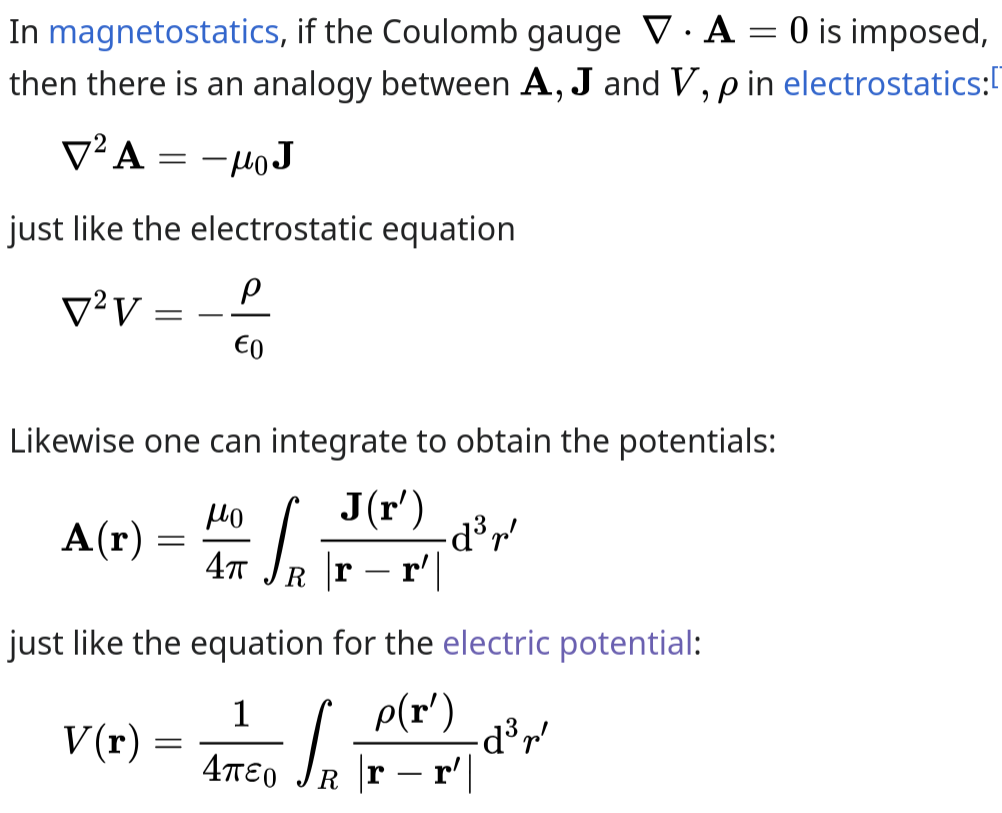
We want to do the same thing for the magnetic field. We know that $B$ is build from currents via the biot savard law:
$\vec B \cong \int_{V} \frac{J(x') \times\hat r(x')}{r(x')^{2}} d^{3}x'$
What we do here we go to every current point, from where we stand, and we project the current onto our direction. We then scale back by the inverse square of the distance.
What we would like to find is an object, that precomputes the distance, so we only need to do the cross product later. The object that does this is the vector potential. And at least in the coulomb gague it is also fairly nice.
(stolen from wikipedia)
 This picture directly shows, that $A$ will "point in the direction" of $J$ (or at least some sort of average.) Some people also interpret $A$ as "momentum you could unlock if you had charge". Which we will see later as minimal coupling
We can thus draw the following picture for an infinite wire and an infinite coil
This picture directly shows, that $A$ will "point in the direction" of $J$ (or at least some sort of average.) Some people also interpret $A$ as "momentum you could unlock if you had charge". Which we will see later as minimal coupling
We can thus draw the following picture for an infinite wire and an infinite coil
 ###### Concept question
With that new found interpretation. Explain the form of the fields given the gaugue. Why do they take this particular form?
$E = -\nabla \phi - (\frac{1}{c}\dede{}{t} A)$
$B = \nabla \times A$
#### Sidenote Lorentz Invariance / covariance
## Light matter interactions
### Matter
#### Fermis Golden Rule
We consider an atom, that is subjected to an oscillating potential starting at $t_{0}$
We can write the Hamiltonian as:
$H = H_{0} + H_{I}$
With $H_{I} = V \theta(t - t_{0}) e^{-\omega t} + c.c.$
and $H_{I} \propto \varepsilon \ll 1$
Before $H_{I}$ takes action we have a stable system according to $H_{0}$, we will thus start in a state well described with energy eigenstates of $H_{0}$. $\ket i$
We want to find out how quickly particles move to other states.
For this we introduce the transition rate $\Gamma_{i \to f}$
To make our lives simple we assume that $\ket i$ is always filled back up and $\ket f$ is always directly removed.
We can think of the transition rate as being made from two parts:
1) Energy conservation
2) Overlap matching
Without going through the derivation I will just show you the result:
$$\Gamma_{i\to f} = \frac{2\pi}{\hbar} |\bra f \hat V \ket i|^{2} \delta(E_{f}-E_{i}-\hbar \omega ) + \frac{2\pi}{\hbar} |\bra f \hat V \ket i|^{2} \delta(E_{f}-E_{i}+\hbar \omega ) $$
We first note the $\delta$ terms. They specify that the difference between energy levels needs to match the energy of the wave. (I specifically don't call this a photon yet, because the wave is still modeled classically)
We see that we can have both $\hbar \omega = E_{f}-E_{i}$ (excitation) as well as $\hbar \omega = E_{i}-E_{f}$ (deexcitation).
Additionally we have the overlap terms $\bra f \hat V \ket i$. This quantifies how well the potential "connects" $f \to i$.
We note in particular that this will be very dependent on symmetry.
For all the people that have taken spectroscopy, this is the reason why we can even do spectroscopy. Because it turns out that actually only very few transitions are allowed by symmetry. The types of allowed transitions then gives us a lot of information about the structure of the system we are interacting with.
It also gives us the power to control the state of the system. We can for example preferentially pump atoms into specific states.
> sketch
Which you will learn all about in quantum optics.
### Minimal coupling
We consider a charged particle in a field. We can write the hamiltonian as follows:
$$\hat H = \frac{1}{2m}\left(\hat p - \frac{q}{c}A (\hat x, t)\right)^{2} + q \phi(\hat x,t) + U(\hat x)$$
You have seen this in your exercise sheet, where you also showed that for this thing to be gauge invariant we need to also add a phase to the wave function.
This gives us the tools to understand a very interesting quantum mechanical effect
#### Sidenote Aharonov Bohm effect
Consider an infinite coil, which has a B-field inside, but none outside.
We saw previously that even if there is no $B$ field, we can still have some $A$ outside.
Consider a particle interfering around the coil. One will have the $A$ field push against $p$, where the other will push in the direction of $p$. We would thus expect a phase difference to show up between the two arms. (Which it indeed does :))
#### Interaction hamiltonian
We can decompose the hamiltonian into the uncharged and the charged case. (We will for now remove the potential $\phi$)
We get:
$$H_0 = \frac{p^{2}}{2m} + U$$
$$H_{I} = \frac{-q}{2mc}(pA + Ap) + \mathcal O(A^{2})$$
We introduce the particle current density
$$\hat j(x) = \frac{1}{2m}(\hat p \delta(x - \hat x) + \delta(x - \hat x) \hat p)$$
Note that some variables have hats, while others don't.
The ones with hats always act on the wave function, they will give out a position/ momentum.
The ones without hats (particularly $x$) are for parametrizing $j$. That is we want to know the particle current density at $x$.
For this we need to know what the probability is to find a particle to have a position component $x$.
Or formulated differently. We are wondering about $\delta(x-\hat x) \Psi$.
This object evaluates the projection of $\Psi$ onto $x$ and then maps it to $x$. Essentially it extracts the "probability" of finding the particle at $x$. (it's not really the probability, more like the wave function density)
We can then rewrite our hamiltonian:
$H_{I} = - \frac{q}{c}\int \hat j(x) \cdot A(x) d^{3}x$
Our interaction energy thus measures how much of the probability current follows the vector potential. (The current wants to follow the vector potential).
Note $j$ is not exactly the electric current density.
Fourier transforming this and decomposing the hamiltonian into the different modes we found a very complicated way to build the prerequisites of the FGR.
$$H_{I}= \hat V_{\vec k,\lambda}e^{i\omega_{k}t} + c.c.$$
$$\Gamma_{i\to f}^{k\lambda} = \frac{2\pi}{\hbar} |\bra f \hat V \ket i|^{2} \delta(E_{f}-E_{i}-\hbar \omega ) + \frac{2\pi}{\hbar} |\bra f \hat V \ket i|^{2} \delta(E_{f}-E_{i}+\hbar \omega ) $$
#### The full picture
We now zoom back out and want to see what happens if a wave interacts with our particle.
For that we realize that a wave will have many different wave componets. The total transition rate will thus be the sum of all possible excited transitions:
$$\Gamma_{i\to f} = \sum\limits_{k,\lambda} \Gamma_{i\to f}^{k,\lambda}$$
In free space we will have all possible allowed $k$, we can thus go from sum to integral:
$\sum\limits_{k,\lambda}= \sum\limits_{\lambda} \frac{L^{3}}{(2\pi)^{3}}\int d^{3}k$
We now want to separate into solid angle and $\omega$.
$$= \sum\limits_{\lambda} \frac{L^{3}}{(2\pi c)^{3}} \int d\omega \omega^{2}\int d\Omega$$
This allows us to write a differential transition rate
$$d\Gamma_{i\to f} (\vec n) = \frac{2\pi q^{2}}{\hbar^{2}c^{2}} \frac{\omega_{if}^{2}}{(2\pi c)^{3}} \sum\limits_{\lambda}|a(\vec k,\lambda)|^{2} \cdot |\bra f \vec j(-\vec k) \cdot \vec e(\vec k,\lambda) \ket i |^{2} d\Omega$$
With $a$ the mode amplitude, $j$ the probability current, and $e$ the polarization vector and $\vec n$ the direction the ray is coming in at.
We can try and disentangle the different components:
- First we have prefactors, which scale with charge and frequency.
That means the higher the energy and the larger the charge, the more strongly will we interact. (Note that those scalings are results from the approximations we do)
- We then see that the larger the amplitude of the mode is the more we transition (but only if the field contains the mode $\lambda$)
- We also see that we now have a specific transition element. It shows that the probability current needs to point in the direction of the polarization.
#### Dipole approximation
We will see more details next week, but for now I can show you that for many cases:
$j(-k) = \frac{p}{m}$
Noting that $$[p^{2},x] = p^{2}x - xp^{2} = px^{2}- (px - [p,x])p = p^{2}x - pxp + i\hbar p $$$$
= p^{2}x - p(px - [p,x]) +i\hbar p = 2i\hbar p$$
###### Concept question
With that new found interpretation. Explain the form of the fields given the gaugue. Why do they take this particular form?
$E = -\nabla \phi - (\frac{1}{c}\dede{}{t} A)$
$B = \nabla \times A$
#### Sidenote Lorentz Invariance / covariance
## Light matter interactions
### Matter
#### Fermis Golden Rule
We consider an atom, that is subjected to an oscillating potential starting at $t_{0}$
We can write the Hamiltonian as:
$H = H_{0} + H_{I}$
With $H_{I} = V \theta(t - t_{0}) e^{-\omega t} + c.c.$
and $H_{I} \propto \varepsilon \ll 1$
Before $H_{I}$ takes action we have a stable system according to $H_{0}$, we will thus start in a state well described with energy eigenstates of $H_{0}$. $\ket i$
We want to find out how quickly particles move to other states.
For this we introduce the transition rate $\Gamma_{i \to f}$
To make our lives simple we assume that $\ket i$ is always filled back up and $\ket f$ is always directly removed.
We can think of the transition rate as being made from two parts:
1) Energy conservation
2) Overlap matching
Without going through the derivation I will just show you the result:
$$\Gamma_{i\to f} = \frac{2\pi}{\hbar} |\bra f \hat V \ket i|^{2} \delta(E_{f}-E_{i}-\hbar \omega ) + \frac{2\pi}{\hbar} |\bra f \hat V \ket i|^{2} \delta(E_{f}-E_{i}+\hbar \omega ) $$
We first note the $\delta$ terms. They specify that the difference between energy levels needs to match the energy of the wave. (I specifically don't call this a photon yet, because the wave is still modeled classically)
We see that we can have both $\hbar \omega = E_{f}-E_{i}$ (excitation) as well as $\hbar \omega = E_{i}-E_{f}$ (deexcitation).
Additionally we have the overlap terms $\bra f \hat V \ket i$. This quantifies how well the potential "connects" $f \to i$.
We note in particular that this will be very dependent on symmetry.
For all the people that have taken spectroscopy, this is the reason why we can even do spectroscopy. Because it turns out that actually only very few transitions are allowed by symmetry. The types of allowed transitions then gives us a lot of information about the structure of the system we are interacting with.
It also gives us the power to control the state of the system. We can for example preferentially pump atoms into specific states.
> sketch
Which you will learn all about in quantum optics.
### Minimal coupling
We consider a charged particle in a field. We can write the hamiltonian as follows:
$$\hat H = \frac{1}{2m}\left(\hat p - \frac{q}{c}A (\hat x, t)\right)^{2} + q \phi(\hat x,t) + U(\hat x)$$
You have seen this in your exercise sheet, where you also showed that for this thing to be gauge invariant we need to also add a phase to the wave function.
This gives us the tools to understand a very interesting quantum mechanical effect
#### Sidenote Aharonov Bohm effect
Consider an infinite coil, which has a B-field inside, but none outside.
We saw previously that even if there is no $B$ field, we can still have some $A$ outside.
Consider a particle interfering around the coil. One will have the $A$ field push against $p$, where the other will push in the direction of $p$. We would thus expect a phase difference to show up between the two arms. (Which it indeed does :))
#### Interaction hamiltonian
We can decompose the hamiltonian into the uncharged and the charged case. (We will for now remove the potential $\phi$)
We get:
$$H_0 = \frac{p^{2}}{2m} + U$$
$$H_{I} = \frac{-q}{2mc}(pA + Ap) + \mathcal O(A^{2})$$
We introduce the particle current density
$$\hat j(x) = \frac{1}{2m}(\hat p \delta(x - \hat x) + \delta(x - \hat x) \hat p)$$
Note that some variables have hats, while others don't.
The ones with hats always act on the wave function, they will give out a position/ momentum.
The ones without hats (particularly $x$) are for parametrizing $j$. That is we want to know the particle current density at $x$.
For this we need to know what the probability is to find a particle to have a position component $x$.
Or formulated differently. We are wondering about $\delta(x-\hat x) \Psi$.
This object evaluates the projection of $\Psi$ onto $x$ and then maps it to $x$. Essentially it extracts the "probability" of finding the particle at $x$. (it's not really the probability, more like the wave function density)
We can then rewrite our hamiltonian:
$H_{I} = - \frac{q}{c}\int \hat j(x) \cdot A(x) d^{3}x$
Our interaction energy thus measures how much of the probability current follows the vector potential. (The current wants to follow the vector potential).
Note $j$ is not exactly the electric current density.
Fourier transforming this and decomposing the hamiltonian into the different modes we found a very complicated way to build the prerequisites of the FGR.
$$H_{I}= \hat V_{\vec k,\lambda}e^{i\omega_{k}t} + c.c.$$
$$\Gamma_{i\to f}^{k\lambda} = \frac{2\pi}{\hbar} |\bra f \hat V \ket i|^{2} \delta(E_{f}-E_{i}-\hbar \omega ) + \frac{2\pi}{\hbar} |\bra f \hat V \ket i|^{2} \delta(E_{f}-E_{i}+\hbar \omega ) $$
#### The full picture
We now zoom back out and want to see what happens if a wave interacts with our particle.
For that we realize that a wave will have many different wave componets. The total transition rate will thus be the sum of all possible excited transitions:
$$\Gamma_{i\to f} = \sum\limits_{k,\lambda} \Gamma_{i\to f}^{k,\lambda}$$
In free space we will have all possible allowed $k$, we can thus go from sum to integral:
$\sum\limits_{k,\lambda}= \sum\limits_{\lambda} \frac{L^{3}}{(2\pi)^{3}}\int d^{3}k$
We now want to separate into solid angle and $\omega$.
$$= \sum\limits_{\lambda} \frac{L^{3}}{(2\pi c)^{3}} \int d\omega \omega^{2}\int d\Omega$$
This allows us to write a differential transition rate
$$d\Gamma_{i\to f} (\vec n) = \frac{2\pi q^{2}}{\hbar^{2}c^{2}} \frac{\omega_{if}^{2}}{(2\pi c)^{3}} \sum\limits_{\lambda}|a(\vec k,\lambda)|^{2} \cdot |\bra f \vec j(-\vec k) \cdot \vec e(\vec k,\lambda) \ket i |^{2} d\Omega$$
With $a$ the mode amplitude, $j$ the probability current, and $e$ the polarization vector and $\vec n$ the direction the ray is coming in at.
We can try and disentangle the different components:
- First we have prefactors, which scale with charge and frequency.
That means the higher the energy and the larger the charge, the more strongly will we interact. (Note that those scalings are results from the approximations we do)
- We then see that the larger the amplitude of the mode is the more we transition (but only if the field contains the mode $\lambda$)
- We also see that we now have a specific transition element. It shows that the probability current needs to point in the direction of the polarization.
#### Dipole approximation
We will see more details next week, but for now I can show you that for many cases:
$j(-k) = \frac{p}{m}$
Noting that $$[p^{2},x] = p^{2}x - xp^{2} = px^{2}- (px - [p,x])p = p^{2}x - pxp + i\hbar p $$$$
= p^{2}x - p(px - [p,x]) +i\hbar p = 2i\hbar p$$