$\newcommand{\dede}[2]{\frac{\partial #1}{\partial #2} }
\newcommand{\dd}[2]{\frac{d #1}{d #2}}
\newcommand{\divby}[1]{\frac{1}{#1} }
\newcommand{\typing}[3][\Gamma]{#1 \vdash #2 : #3}
\newcommand{\xyz}[0]{(x,y,z)}
\newcommand{\xyzt}[0]{(x,y,z,t)}
\newcommand{\hams}[0]{-\frac{\hbar^2}{2m}(\dede{^2}{x^2} + \dede{^2}{y^2} + \dede{^2}{z^2}) + V\xyz}
\newcommand{\hamt}[0]{-\frac{\hbar^2}{2m}(\dede{^2}{x^2} + \dede{^2}{y^2} + \dede{^2}{z^2}) + V\xyzt}
\newcommand{\ham}[0]{-\frac{\hbar^2}{2m}(\dede{^2}{x^2}) + V(x)}
\newcommand{\konko}[2]{^{#1}\space_{#2}}
\newcommand{\kokon}[2]{_{#1}\space^{#2}} $
# Content
$\newcommand{\L}{\mathcal L}$
## Feedback
Thanks for the feedback last week!
In general the speed an level of the lecture are good, which is nice to hear.
However I heard from a lot of you that you'd prefer to stay closer to the lecture. I hear you and I'll try to do a concrete lecture recap at the beginning of every lesson.
However due to the rather slow progression of the lecture I will probably not be able to fill the full two lectures with just repetition.
I have the following suggestion:
- First lecture: Extra content around the lecture
- Second lecture: Repetition & QnA
I'll reserve 15 min at the end of the lecture for you to ask me questions.
This week will be a bit repetition heavier because I'll try to recap the chapter of path integrals.
## This week
### Repetition Theory of heat
#### Entropy
In theory of heat you have seen three characterizations of entropy:
- Thermodynamic
- Statistical
- Informational
They all had differing interpretations, but ended up being the same thing.
##### Thermodynamic
Thermodynamic entropy was defined via the heat $\delta Q = TdS$
Combining this with $dU = dQ + dW = TdS + dW$
And considering a system which does not accept energy $dU = 0$
We get:
$-\dd{W}{S} = T$
The Temperature is the conversion factor of entropy to work. I.e Entropy is in some sense a measure for how much "usable work" is inside a system. Per $dS$ entropy produced at temperature $T$, we get a $dW$ of work out of the system.
##### Statistical
$S = k_{B}\ln(\Omega)$
Where $\Omega$ is the number of microstates.
Here we interpret entropy as "disorder". We can try and bridge this to the thermodynamic interpretation by taking the total derivative:
$dS = \frac{k_{B}}{\Omega}d\Omega$
What this shows is that as we increase entropy, we also increase the number of states. This means by extracting work via a system we need to allways add more states to some other system.
I.e. to extract work from a machine, the machine needs to "mess up" some part of the environment (or itself, but then it wouldn't be that good of a machine)
##### Informational
The last interpretation of entropy you might have seen is the information entropy.
Which you found via
$\frac{E}{T}\geq k_{B}\ln(2)$
Which is a bound on how cheaply you can reset a bit.
The identification with entropy is straight forward by plugging in $\Omega = 2$ (for a bit).
The interpretation can be done either via the thermodynamical entropy, by imagining that you have to localize a single particle on either the left or the right half of a volume.
For this you need to compress the volume to half the size (doing work.)
If you do the math you find the bound.
Alternatively you can say that knowing the exact microstate of a system allows you to extract work via "maxwells daemon".
##### Summary
We see that the information about a system, and the energy extractable from that system, and the number of states a system has are tightly interwoven.
We will try to extend this understanding to quantum particles.
#### Gibbs (canonical) ensemble
In theory of heat you should have seen how we can describe the thermal occupation of a system using its partition function $Z$.
Specifically we had $p_{\mu}= \frac{1}{Z}e^{\frac{-E_{\mu}}{k_{B}T}} = \frac{1}{Z}e^{-\beta E_\mu}$
With $\beta = \frac{1}{k_{B}T}$ the inverse temperature. And $Z$ the partition function, which was mainly a normalization constant.
From this formula we see that $k_{B}T$ is the "typical energy scale" of a system at temperature $T$. Meaning that if a energy jump is $\approx k_{B}T$ it can be thermally done, if its more than that it is exponentially suppressed.
We wanted our probabilities to add to one so we had:
$\sum\limits_{\mu} p_{\mu} = 1$
$\sum\limits_{\mu} \frac{1}{Z} e^{-\beta E_{\mu}} = 1$
$Z = \sum\limits_{\mu}e^{-\beta E}$
If you remember there were different ensembles, which all held different external _macroscopic_ variables fixed.
In the case of the Gibbs (canonical) ensemble those variables were:
($N$, $T$,$V$)
### Repetition QM
#### Pure vs mixed
(note I left out all the normalisation factors)
Consider: $\ket \psi = \ket \uparrow + \ket \downarrow$ (a pure state) $\rho = \ketbra \psi \psi$
We also consider the computational basis
- $\ket + = \ket \uparrow + \ket \downarrow$.
- $\ket - = \ket \uparrow - \ket \downarrow$.
I.e we get something like:
$\ket \uparrow = \ket + +\ket -$
$\ket \downarrow = \ket + -\ket -$
So for our state $\ket \psi = (\ket + + \ket -) + (\ket + - \ket -) = \ket +$
If we now measure along the $\uparrow \downarrow$ basis, we will get $50:50$ $\uparrow$ or $\downarrow$.
If we measure along the $+/-$ basis however, we will always get $+$
We might think this state is just in a statistical mixture of $\uparrow$ and $\downarrow$
So we compare with a mixed state $\rho = \ketbra \uparrow \uparrow + \ketbra \downarrow \downarrow$
If we measure $\uparrow \downarrow$ we will get $50:50$ $\uparrow$ and $\downarrow$ as expected.
But if we measure in the $+/-$ basis we will get the following:
First consider $\ketbra \uparrow \uparrow$
$$\ketbra \uparrow \uparrow = (\ket + + \ket -)( \bra + + \bra -) = \ketbra ++ + \ketbra -- + \underbrace{(\ketbra +- + \ketbra -+)}$$
then consider $\ketbra \downarrow\downarrow$
$$\ketbra \downarrow \downarrow = (\ket + - \ket -)(\bra + - \bra -) = \ketbra + + + \ketbra - - - \underbrace{(\ketbra +- +\ketbra -+)}$$
The crossterms $\ketbra \pm \mp$ will cancel.
We get $\rho = \ketbra ++ + \ketbra --$
Meaning if we measure $\rho$ in the $+/-$ basis, we will get $50:50$ $+/-$. (Not the $100\%$ $+$)
> Long story short: The difference between mixed and pure states is, that a pure state has a basis, in which it is well defined.
> A Mixed state is "random" from every direction, no matter in which basis I measure.
### Thermodynamic path integrals:
In the lecture you saw that you can derive path integrals that represent thermodynamic expectation values.
#### Outline:
1) Find quantum statistical ensemble via diagonal matrix elements
2) Distribute the statisticalness ($e^{-\beta H}$) to the operator (a bit like heisenberg picture)
3) Change into a (for now) arbitrary position basis
4) Realize that the result looks like a path integral with the exception, that the exponential is real instead of imaginary
5) Identify the cyclical path integral
6) Profit
#### Step by step
##### 1)
First we note that classically we would expect a probability distribution of the shape $p_{\mu}= \frac{1}{Z}e^{-\beta E_{\mu}}$
Now if we consider some observable $A$
We can say that we expect to find a statistical mixture of measurement outcomes.
$\langle A \rangle_{\beta}= \frac{1}{Z}\sum\limits_{k} e^{-\beta E_{k}} \bra E_{k} A \ket E_{k}$
That is we make a statistical mixture between measuring along the specific eigenvectors
##### 2)
For now $e^{\ldots}$ is just a number, we can move it around
$\langle A \rangle_{\beta}= \frac{1}{Z}\sum\limits_{k} \bra E_{k}e^{\frac{-\beta}{2} E_{k}} A e^{\frac{-\beta}{2} E_{k}}\ket E_{k}$
We now realize that we paired eigenenergies with eigenstates, we can "reverse" the normal procedure, where we go from $H\psi \to E\psi$
and write
$\langle A \rangle_{\beta}= \frac{1}{Z}\sum\limits_{k} \bra E_{k}e^{\frac{-\beta}{2} H^{\dagger}} A e^{\frac{-\beta}{2} H}\ket E_{k}$
(note that $H = H^{\dagger}$)
##### 3)
We note that sum over a complete set of basisvectors ($\ket E_{k}$) is a trace, and can be replaced by any other complete set of basisvectors.
We arbitrarily choose $q$. The sum becomes an integral
$$\langle A \rangle_{\beta}= \frac{1}{Z}\int \bra q e^{\frac{-\beta H}{2}}A e^{\frac{-\beta H}{2}} \ket q dq$$
##### 4)
Now we do something really strange....
We note that the expression $\bra q \ldots \ket q$ looks really familiar.
Remember the correlation function:
$\bra{q,t_{f}} A_{H}(t) \ket{q,t_{i}} = \int_{\gamma}D\gamma A(q) e^{\frac{iS[\gamma]}{\hbar}}$
We can now deconstruct the expression. Where we switched back to the Schrödinger picture with $A$
$$\bra{q,t_{f}} A_{H}(t) \ket{q,t_{i}} = \bra{q} U(t_{f},t) AU( t,t_{i})\ket{q} $$
If we want the expression inside of the integral to match we need:
$U(t_{f},t) = e^{-\beta \frac{H}{2}} = U(t, t_{i})$
$e^{\frac{1}{i\hbar}(t_{f}-t)H} = e^{-\beta \frac{H}{2}} = e^{\frac{1}{i\hbar}(t-t_{i})H}$
$t_{f}-t = -i\hbar \frac{\beta}{2} = t-t_{i}$
We don't need the variable $t$, so we set it to zero
$t_{f} = \frac{-i\hbar\beta}{2} = -t_{i}$
We find that we need to integrate over _imaginary_ times match the two notions.
We also note that $q_{i}=q_{f}$ thus all our paths that we will consider are cyclical.
##### 5
Putting everything together we get
$$\langle A\rangle_{\beta} = \frac{1}{Z}\int \underbrace{\bra{q,\frac{-i\hbar\beta}{2}} A \ket{\frac{i\hbar\beta}{2}, q}}_{\substack{\text{Correlation function (q to q).}\\ \text{ Starting at } t_{i}=\frac{i\hbar\beta}{2} \\ \text{and ending at } t=\frac{-i\hbar\beta}{2} }} dq = \frac{1}{Z}\int dq \int_{\substack{q\to q \\ \frac{i\hbar\beta}{2} \to \frac{-i\hbar\beta}{2}}} D\gamma A(q) e^{\frac{iS[\gamma]}{\hbar}}$$
We thus find that if we do the cyclical path integral over imaginary time at every point, we get the expectation value of an observable $A$
##### 6
Profit?
Well integrating over complex time is... strange.
So we actually instantly get rid of complex time.
We introduce the euclidian time $\tau = i t$, which has the only purpose of making our integrals real again.
We find that we also need to adjust our action $S$ (remember by pure units $S$ is a $dt$ integral of $L$. Thus making $t$ complex will also make $S$ complex)
We find $S_{E}[\gamma_{E}] = -iS[\gamma]$
##### 7
Profit!
$$\frac{1}{Z}\int dq \int_{\substack{q\to q \\ \frac{i\hbar\beta}{2} \to \frac{-i\hbar\beta}{2}}} D\gamma A(q) e^{\frac{iS[\gamma]}{\hbar}} = \frac{1}{Z} \int dq \int_{\substack{q\to q \\ -\frac{\hbar\beta}{2} \to \frac{\hbar\beta}{2}}} D\gamma_{E}A(\gamma_{E}(0))e^{\frac{-S[\gamma]}{\hbar}}$$
This is a normal cyclical path integral that take the time $\hbar \beta$.
We then do this for every position and we get the expectation value of $A$
## Repetition Path integrals
Today we will actually have a bit more repetition than normally, because we now have enough of the lecture covered to do a full recap of the story, concepts and ideas behind the path integral formalism.
### Historical motivation & classical analogy
We found that we wanted an alternative quantisation than the canonical quantisation. This was mainly motivated by the fact that we wanted to do quantum for integrals, not just states.
For this we remembered the Lagrangian formalism, where extremalizing the Action $S[\gamma]$ leads to a physical path.
The action was given as the path integral over the Lagrangian $\L = T-V$
To quantize the Lagrangian formalism, we first had to quantize paths.
### The propagator kernel
For this we looked at the propagator kernel $K = \bra q_{f}U \ket q_{i}$. It gave us a probability to transition from $i \to f$ in time $\Delta t$
We then further looked at what happens if our $U$ restricts our possibilities. For this we considered a slit at $q$.
We found that if we consider the superposition of all slits, we recover the no-slit limit.
What we essentially said is:
> If we allow the combination of all possible restrictions, we are no longer restricted.
We then realized that we can actually do this "superposition of slits" at every subdivision of our path. We also realized that at every new subdivision we could choose a new slit to pass through.
The combination of choosing a different slit at every time subdivision gave us a combination of paths!
$$K(t_{f}-t_{i},q_{f}) = \int dq_{1} \cdots \int dq_{N-1} K(\epsilon, q_{f},q_{N-1} K(\epsilon, q_{N-1}, q_{N-2}) \cdots K(\epsilon, q_{1},q_{i}))$$
We then realized that for very small timesteps we can evolve the particle by quickly switching between "potential evolution" and "kinetic evolution".
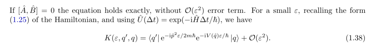 We supported that intuition via the BCH formula.
Having split kinetic and potential evolution, we used the fourier transform to do the kinetic evolution explicitly.
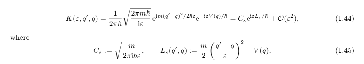
We found that we need to evaluate this gaussian integral $e^{p^{2}}$
We thus found an explicit formula for $K$ in the $t\to \varepsilon$ limit. We identified it with the _classical_ lagrangian!
We supported that intuition via the BCH formula.
Having split kinetic and potential evolution, we used the fourier transform to do the kinetic evolution explicitly.
We found that we need to evaluate this gaussian integral $e^{p^{2}}$
We thus found an explicit formula for $K$ in the $t\to \varepsilon$ limit. We identified it with the _classical_ lagrangian!
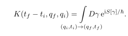
 ### The path integral
Because we now had a formula for $K$ given in exponentials, and we had an integral over all possible slits at every subdivision.
We realized that we can use the exponential rules, to transform a multiplication of the $K$ to a sum of the $L's$
### The path integral
Because we now had a formula for $K$ given in exponentials, and we had an integral over all possible slits at every subdivision.
We realized that we can use the exponential rules, to transform a multiplication of the $K$ to a sum of the $L's$
 Again taking the limit $\varepsilon \to 0$ and $N \to \infty$ we found that the exponential is actually just the action $S[\gamma]$
We thus found the path integral:
Again taking the limit $\varepsilon \to 0$ and $N \to \infty$ we found that the exponential is actually just the action $S[\gamma]$
We thus found the path integral:
 ### Applications
### The classical limit
### Commutation & Time ordering
### Applications
### The classical limit
### Commutation & Time ordering